A PID controller simulation in a Haskell
I stumbled onto a Haskell DSL called Copilot for building software health monitors in embedded systems.
The physical part of a cyber-physical system is continuous, so infinite streams of data are good models for their inputs. Consider an autopilot in a plane. It it might sample an altitude sensor periodically, but it needs to keep doing that for an unknown amount of time (until the plane lands). It can’t buffer data, it needs to handle each sample as it arrives.
Copilot makes it simple to use infinite sampled data streams in Haskell. External streams represent the sensor (or other) data coming into the monitor. A spec is the container around the monitor, the trigger, and the streams. The trigger is the function to call when the monitored condition occurs.
The idea of infinite samples streams reminded me of Simulink, so I decided to build a PID controller simulation.
Below is my spec, simplified for clarity:
impulseResponse :: Spec
impulseResponse = do
  observer "y" (y)
  trigger "danger!"
    (maxErrExceeded) []
The name of the spec is impulseResponse, my trigger function to call is called danger! and my monitoring condition is maxErrExceeded. Observers are used to monitor the value of the streams. The have the form:
observer "description" (variable_name)Where description can be any string you want. It appears as the column header in the output when the spec is interpreted. I monitor almost all the variables in the real version for plotting.
I defined normal float variables for the coefficients of my PID controller:
p = 0.5   -- P term coefficient
i = 0.2   -- I term coefficient
d = 0.2   -- D term coefficient
Now I need to define streams for the requested input y, the commanded output u and the error e:
y :: Stream Double    -- controller input
u :: Stream Double    -- controller output
e :: Stream Double    -- error between input and output
For a real PID controller I also need to know the derivative for the error and the integral:
integral :: Stream Double     -- integral of the error
dedt :: Stream Double         -- derivative of the error
Calculating the streams is the fun part. The input y is the most straightforward. All I wanted was an impulse, so I made an infinite stream of ones and added some zeros at the beginning:
y = [0.0, 0.0, 0.0, 0,0] ++ 1.0 -- input is an impulseFor u, the initial command is 0.0, but the other commands need to be calculated:
u = [0.0] ++ command -- the PID controller outputError is just input minus output
e = y - u -- the error streamAdding a zero in front of a stream has the effect of “delaying” it one tick. To calculate the derivative of the error, I delay the error stream one tick and subtract it from itself:
dedt = e - ([0.0] ++ e)The integral just adds the error to itself for each tick:
integral = [0.0] ++ integral + eAll the streams are defined, so I just define a PID controller in the textbook way:
command = u + e * p + integral * i + d * dedt -- a tradition PID controllerThe condition I want to monitor is the size of the error. I just picked a random value of 0.2. (It should really monitor the absolute value of the error).
maxErrExceeded :: Stream Bool
maxErrExceeded = e > 0.2 -- the condition to monitor
For output I just observed the variables I was interested in and interpreted my spec the normal Copilot way:
interpret 50 impulseResponseThis runs my simulation and tells me when the trigger happens (and what the value of the observed streams are, if any). I put the output into a .txt file and graphed it with a python script (see end of post for code).
As a simple first test, I tried P = 0.5, I = 0.0, D = 0.0. This is not really
a PID controller, but just a P controller. Here’s what I got:
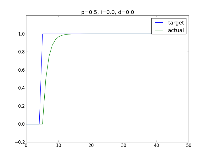
Ahh, the good old P term. He’s slow but he’s reliable. The P=0.5 controller isn’t half bad if you ask me.
For a cooler graph, I used P=0.5, I=0.2, D=0.2:
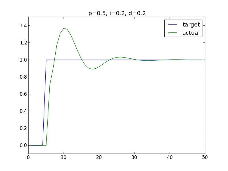
Now, that looks like something from my Control Systems textbook.
This is the end. A simulation of a PID controller over infinite streams written in Haskell is pretty cool if you ask me.
Here’s my complete code:
impulse.hs:
import Language.Copilot
import qualified Prelude as P

impulseResponse :: Spec
impulseResponse = do
  observer "dedt" (dedt)
  observer "int." (integral)
  observer "y" (y)
  observer "u" (u)
  observer "e" (e)
  trigger "danger!"
    (maxErrExceeded) []
  where

  p = 0.5   -- P term coefficient
  i = 0.2   -- I term coefficient
  d = 0.2   -- D term coefficient

  y :: Stream Double -- controller input
  u :: Stream Double -- controller output
  e :: Stream Double -- error between the input an output
  integral :: Stream Double -- integral of the error
  dedt :: Stream Double -- derivative of the error

  y = [0.0, 0.0, 0.0, 0,0] ++ 1.0 -- input is an impulse
  u = [0.0] ++ command
  e = y - u
  dedt = e - ([0.0] ++ e)
  integral = [0.0] ++ integral + e

  command = u + e * p + integral * i + d * dedt -- a tradition PID controller

  maxErrExceeded :: Stream Bool
  maxErrExceeded = e > 0.2 -- the condition to monitor
graphcont.py:
import numpy as np
from pylab import *

if __name__ == '__main__':
    ion()
    f = open("cont.txt")
    y = []
    u = []
    e = []
    intg = []
    for i, line in enumerate(f):
        if i != 0:
            s = line.split()
            #print s
            y.append(double(s[-1]))
            u.append(double(s[-2]))
            #e.append(double(s[2]))
            #intg.append(double(s[3]))
    #print y, u
    figure(1); clf()
    plot(y)
    plot(u)
    ylim(-0.1, 1.5)
    legend(["target", "actual"])
    title("p=0.5, i=0.2, d=0.2")
    show()