The most popular R packages, according to RStudio
I’ve been thinking about doing some empirical R research lately. The nice thing about doing research related to R, is it’s a language people other than computer scientists actually use. In that vein, I decided to try to determine what R packages are the most popular. This isn’t as straightforward as it might seem. The main “official” package archive is CRAN, but there’s also Bioconductor, and probably some others I don’t know about. CRAN has multiple mirriros so there is no one place where the download statistics are kept. The largest compiled statistics I found were at cran-logs.rstudio.com.
RStudio is an IDE for R with many (thousands) of users and they publish their download logs online. The users of RStudio might not be a representative sample of the whole R user population, but that’s the data I have.
I wrote an R script to download the logs and make some nice plots.
First, I wrote two functions to download the logs. I didn’t want to re-download the logs each time, I’ve been working on my local library’s sketchy WiFi lately, so I take the set difference of what I have in my log directory and what RStudio has on its server.
    getMissingLogs <- function() {
        #see http://cran-logs.rstudio.com/
        setwd(LOGDIR)

        # Here's an easy way to get all the URLs in R
        start <- as.Date('2014-06-01')
        today <- as.Date('2014-06-16')

        all_days <- seq(start, today, by = 'day')

        year <- as.POSIXlt(all_days)$year + 1900
        existing_files <- tools::file_path_sans_ext(dir(), TRUE)
        existing_days <- as.Date(existing_files)
        missing_days_raw <- setdiff(all_days, existing_days)

        # it loses the date format for some strange reason
        as.Date(missing_days_raw, origin="1970-1-1")
    }

    syncLogs <- function(missing_days) {

        if (length(missing_days) > 0) {
            setwd(LOGDIR)

            year <- as.POSIXlt(missing_days)$year + 1900
            urls <- paste0('http://cran-logs.rstudio.com/', year, '/', missing_days, '.csv.gz')
            destFiles <- paste0(missing_days, '.csv.gz')

            for (i in 1:length(urls)) {
                download.file(urls[i], destFiles[i], "wget")
                gunzip(destFiles[i])
            }
        }
    }
Now that I’ve downloaded the files, I just open them and merge the tables.
    countPackages <- function() {
        setwd(LOGDIR)
        logs <- dir()
        for (i in 1:length(logs)) {
            df <- read.csv(logs[i])
            t <- table(df[["package"]])
            if (i == 1) {
                counts <- t
            } else {
                counts <- mergeTables(counts, t)
            }
        }
        write.csv(counts, file="../counts.csv")
        sort(counts, decreasing=TRUE)
    }

    mergeTables <- function(a, b) {
        n <- intersect(names(a), names(b))
        c(a[!(names(a) %in% n)], b[!(names(b) %in% n)], a[n] + b[n])
    }
On to the good part. I made two plots to visualize the most popular packages.
plotResults <- function() {
    jpeg("wordcloud.jpg")
    d <- read.csv("countsSorted.csv")
    wordcloud(d[["X.1"]], d[["x"]], max.words=100)
    dev.off()
}
This is a legitimate use for a word cloud; I contend. DBI stands for “Database Interface.” Rcpp is a package for call C++ from R. It’s not surprising the the most popular packages are for the things people typically do in R, namely look at data and plot it. I’m a little surprised the Rcpp is very popular. I thought most R users just used premade packages. Maybe Rcpp is requried by packages they use and they’re not really writting their own.
Now for a more sensible plot, a bar plot.
hbarPlot <- function() {
    jpeg("hbar.jpg")
    d <- read.csv("countsSorted.csv")
    par(las=2) # make label text perpendicular to axis
    range <- 25:1
    barplot(d[range, 3], horiz=TRUE, names.arg=d[range, 2], cex.names=0.7)
    dev.off()
}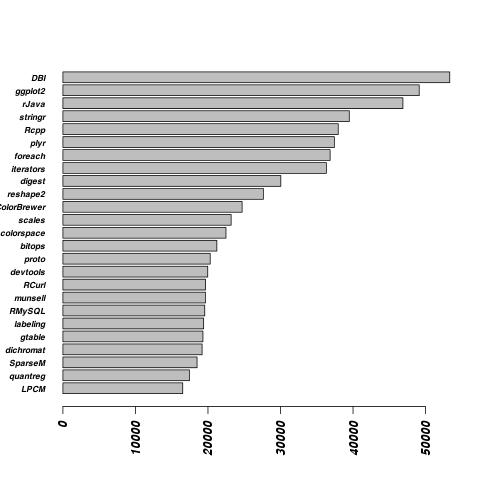
For this plot I can see that sample size actually fairly large. From the begining of June to June 17th, the DBI package was downloaded over 50,000 times.
Tip ‘o the hat to this blog post for pointing me to the RStudio logs.