The most popular R packages are, mostly, written in R
I’ve been starting to think about some R related research. Building on my previous post, wherein I data mine the RStudio logs to find the most popular R packages, I’ve dug a little deeper in to the package contents.
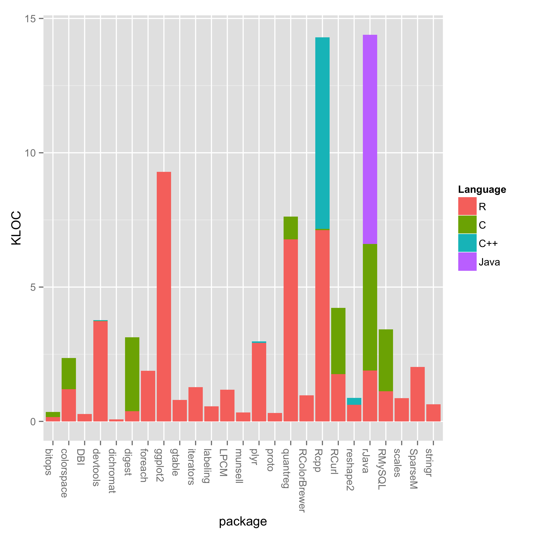
One question I have is, “How much of R is written C/C++ or Fortran?” I expected the performance critical parts, especially linear algebra, to be written in a “faster” language. However, looking at just the top 25 most popular packages, a lot of R is written in R.
Now, the most popular packages don’t represent everything people think of as being R. But the conflation of the R language, the R virutal machine, the base packages, and the contributed packages is really what most people think of as being “R.” This post only looks at a piece of the bigger R ecosystem, but I’ll get to the rest in due time. I should also note these are the most popular non-default packages. For the default packages, which are included with the R installer, I don’t know of a way of measuring their popularity.
Looking at the plot, most packages consist mainly of R code. Notable expections are Rcpp and rJava, which have a lot of C++ and Java code respectively. There’s also a smattering of C across some packages. Some of these are wrappers around C programs such as RCurl, but there could be some C for performance sake. A deeper dive is necessary to deterimine why an individual package uses C.
How did I get this data? In my previous post, I mined the RStudio logs to find the most popular packages. Then I downloaded the packages from CRAN, and ran cloc on them. Note for reproducibility: I had to get the latest-and-greatest cloc from SVN for R support. Luckily cloc has a csv output option, so getting the data into R is as simple as:
cloc <- function(file) {
    nHeader <- 4
    nFooter <- 3
    cmd <- paste0("cloc --force-lang=R,r --csv ", file)
    output <- system(cmd, intern=TRUE)
    output <- output[-(1:nHeader)]
    con <- textConnection(output)
    d <- read.csv(con)
    d <- d[-length(d)] # the last column is some weird string
    languages <- d[["language"]]
    df <- data.frame(t(as.numeric(d[["code"]])), basename(file))
    colnames(df) <- c(as.character(languages), "package")
    return(df)
}
Now I can accumulate the cloc for the top N packages using Map/Reduce:
clocTopN <- function(N) {
    topN <- getTopN(DLCSV, N)
    files <- paste0(EXDIR, topN)
    clocs <- Map(cloc, files)
    merged <- Reduce(function(x, y){merge(x, y, all=TRUE)}, clocs)
    merged[is.na(merged)] <- 0
    return (merged)
}
Then I stash the intermediate results in a file. This function opens the file and makes a nice stacked barplot showing the KLOC (thousands of lines of code) for the various languages in each package.
stackedBarPlot <- function(filename) {
    x <- read.csv(filename, row.names=1)
    langs <- c("R", "C", "C..", "Java")
    displangs <- c("R", "C", "C++", "Java")
    y <- x[c("package", langs)] # get only the columns we want
    y[langs] <- y[langs] /1000 # convert to KLOC
    df <- data.frame(y)
    colnames(df) <- c("package", displangs)
    m <- melt(df, id.vars="package")
    colnames(m) <- c("package", "Language", "KLOC")
    ggplot(m, aes(x = package, y = KLOC, fill = Language)) +
      geom_bar(stat = "identity") +
      ylab("KLOC") +
      theme(axis.text.x = element_text(angle=-90, hjust=0))
    ggsave(file="pkg_comp.png")
}
Making the chart was honestly the hardest part. I’ve used MATLAB and Python’s Matplotlib a lot so R’s plotting is forgein to me. The built-in R plotting seems horrendous, since I am used to plotting that “just works” in MATLAB. But maybe I learned MATLAB so long along that I’ve forgetten how difficult it was to learn. I’ll be trying to learn ggplot2 for future work.